Arithmetic Algorithms

divide and conquer strategy:

breaking the problem into subproblem with the same type
recurssively solve them
glue together the solution

multiplication

(a+bi)(c+di)=
(ac-bd)+(bc+ad)i in this way four multiplication
(ac-bd)+((a+b)(c+d)-ac-bd)i just three ,when recurssively applied,can reduce its calculation
$T(n)=3T(\frac{n}{2})+O(n)$
we can understand it using the call tree
it has the depth of $log_2n$ ,when apply trick,three leaves from single parent node
$3^k\times O(\frac{n}{2^k})$
alt text

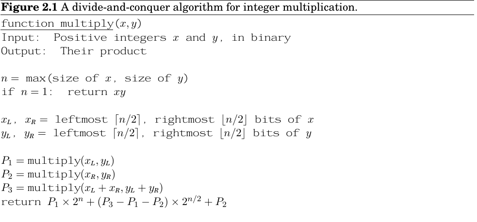
recurrence relation

generic pattern:when solving problem with size n,recurrsively divide it into a subproblems of size $\frac{n}{b}$ ,then conbine in $O(n^d)$
$T(n)=a\times T(\lceil\frac{n}{b}\rceil)+O(n^d)$
$T(n)= \begin{cases} O(n^dlogn) & \frac{a}{b^d}=1\\\\ O(n^d) & \frac{a}{b^d}<1\\\\ O(n^{log_ba})& \frac{a}{b^d}>1\\\\ \end{cases}$

mergesort & median

iterative mergesort:
maintain a queue of active arrays,each time dequeue the two arrays and merge,enqueue the result,until the queue has one array
randomized divide-and-conquer selection
- step1:chose a value v,split array into SL,SV,SR three part (less,equal,bigger)
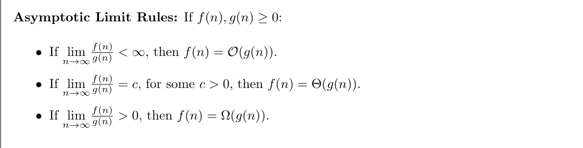
- step2: $selection(S,K)=\begin{cases}selection(SL,K)&K\le |SL|\\\\ v & |SL|<K\le |SL|+|SR| \\\\ selection(SR,K-|SL|-|SV|)& K>|SL|+|SR| \end{cases}$

efficiency analysis:

define:the v lies in the percentile of 25%~75% of the array to be good(on average,every two toss can get a coin head)
- which leads to the SL and SR at most of length $\frac{3}{4}$ of original,and the event occurs with 50% probability
  $T(n)=T(\frac{3n}{4})+O(n)=>T(n) \le T(\frac{3n}{4})+Kn$ 展开

dis&hw1

climb step,one step or two step each time
ordinary solution:DFS,runtime exceed polynomial,proof $T(n)=T(n-1)+T(n-2)+1 \gt 2T(n-2)$
one change:maintain an array of computed output
the other
$\begin{bmatrix}f(n)\\\\f(n-1)\end{bmatrix}=\begin{bmatrix}1&1\\\\1&0\end{bmatrix}\times\begin{bmatrix}f(n-1)\\\\f(n-2)\end{bmatrix}$
alt text

way to solve:
1.unraveling:plug in smaller equation
2.draw a tree
3.squeeze:compute its upper and lower bound
e.g:
$T(n)=3T(n^{\frac{1}{3}})+O(logn)$
let x=logn
$S(x)=3S(\frac{x}{3})+O(x)$

fast matrix multiplication

$XY=\begin{bmatrix}A&B\\\\ C&D\end{bmatrix}\times \begin{bmatrix}E&F\\\\ G&H\end{bmatrix}=\begin{bmatrix}P_5+P_4-P_2+P_6&P_1+P_2\\\\ P_3+P_4&P_1+P_5-P_3-P_7\end{bmatrix}$
where
$P_1=A(F-H) \hspace{2em} P_5=(A+D)(E+H)\\\\ P_2=(A+B)H \hspace{2em} P_6=(B-D)(G+H)\\\\ P_3=(C+D)E \hspace{2em} P_7=(A-C)(E+F)\\\\ P_4=D(G-E)$

graph

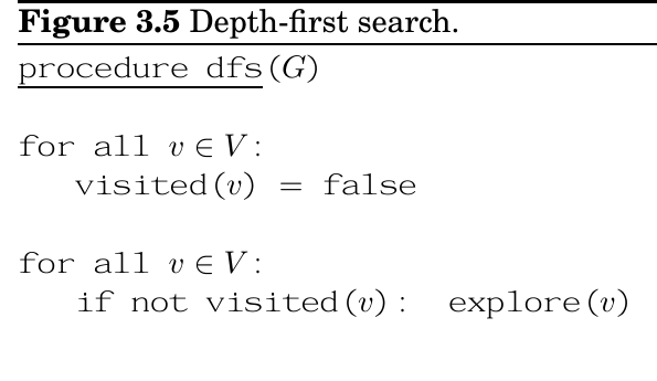
depth first search

form a tree,visited edge are tree edges,unvisited are back edges
(in undirected graph,while in directed graph,back edges point to anscestor(in a single DFS tree),forward point from anscestor,neither called cross edges)

runtime of DFS:marking spots and work on each vertex(O(|V|)),exam the adjacent list (O(|E|)),so total be O(|V|+|E|)
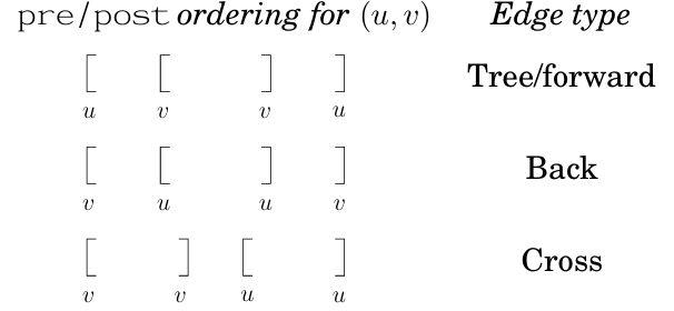
previsit and postvisit ordering:number the time step of previsit and posivisit at the same time
we can discover that for any two nodes u and v [pre[u],post[u]] and [pre[v],[post[v]]] are either disjoint or one contains in other

in directed graph:ancestor vesus descendant

elaborate taxonomy beside tree edges and back edges:
- forward edges:towards the non-child descendant node
- cross edges:towards neither ancestor nor descendant(in the spanning tree)

directed acyclic graph(dag)

property:a directed graph has a cycle if and only if its depth-first search reveals a back edge
property:in a dag,every edge leads to a vertex with lower post number(the vertex won’t be post numbered until recurse end)
- acyclicity,linearizability,the absence of back edge are in fact the same things
property:every dag has at least one source and one sink
- this form an algorithm:find the source and delete edge without in-edge every time

strongly connected component

in directed graph,connectivity between u,v means there exsit pathes from u to v and from v to u

property:every directed graph is a dag of its strongly connected components(a cycle would be merged)

decomposition algorithm

property:if explore start at a node u,then it will terminate when all the node reachable from u visited
- therefore the explore node at the SCC which is a sink in the meta-graph(reduced graph)will exactly traverse the whole SCC
property:the node that receives highest postnumber in DFS must in the source SCC
property:if both A and B are SCC,and there is an edge from node in A to B,then the highest postnumber in A is bigger than B
- this can be restated as SSC can be linearized by decreasing order of their highest postnumber
algorithm:
- run DFS on $G^R$ (the reverse of graph)
- run undirected connected component algorithm,process node in the order of descending of highest postnumber
  - the algorithm on undirected is just DFS,每次explore的时候增加编号

crawling:in the World Wide Web,we don’t know how much node,so

we can’t for adj list,just use stack
no recurssion,explicit stack(启发式,给page rank等最高的最高优先级)
use hashing instead of visited array

disc&hw2

统计逆序数:归并同时计数count(Array)=count(L)+count®+intersect(L,R)
where count()返回数组内的逆序数,intersect统计两者之间的
recurssion分析法,相信sub内已经完成我们想要的保证
bogosort:每次检查是否排序成功,不成功就shuffle,服从几何分布
随机选择枢轴量的quick sort:

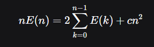
写n-1时的式子两者相减
调和级数 $\sum_{i=1}^{n}\frac{1}{i}=ln n$
在快排中,两个元素A,B发生比较当且仅当第一个从A到B的有序序列中选取的pivot为A或B
最近曼哈顿距离algorithm
- sort by x-coordinate
- divide into L and R,recursively solve minL,minR, $\delta=min(minL,minR)$
- 构造与x中位数差值在 $\delta$ 以内的条带,按y排序,对每个点比较后面常数个点(从下往上找,并且只需要找小于delta的点对，这是常数个)
divide:统计每个内部+各个之间的交互
二分查找的前提是整个array有序,不一定成立!!!灵活一点(矩阵列之间有关系直接用)

You are playing a party game with n other friends, who each play either as a werewolf or a
villager. You do not know who is a villager and who is a werewolf, but all your friends do.
But you know that there are more villagers than there are werewolves. And you also know
that villagers always tell the truth, while werewolves may lie or tell the truth.
Your goal is to identify one player who is definitely a villager. Your elementary query is to
pair up two people and ask each whether the other is a villager or werewolf. Your algorithm
should work regardless of the behavior of the werewolves.

分治方法:分成两堆(村民总数超过一半故至少有一堆的村民超过一半,所以两个一半选出来的村民至少有一个是真的,再全体投一遍)
“候选人法”:两个人都评价:都说是狼人则至少一个是狼人,去掉这对,剩下的人中村民还是严格多于狼人,最后验证

path in graphs

DFS: $O(|V|+|E|)$
对无权图:DFS就能直接找出最短路径
带正权:

可以调整一下,把权重为l的边拆成l条单位权重的边并且插入l-1 个dummy node
dijkstra:想象一个clock,表示估计BFS到达的时间,搜索每到一个节点就更新所有邻接点的估计时间
- 另一种derivation:single-extend of present shortest path(下一步加入的点一定是从已知区域深一步的最短点)
- 形式和DFS一致,但是优先队列的操作开销无法忽略, $O((|V|+|E|)log|V|)$ (binary heap)
- 实际计算公式为

$O(|V|)\times T_{deletemin}+O(|V|+|E|)\times T_{decreasekey}$

- d-ary heap就是d叉树形状的堆,在稠密和稀疏图上效果都还行

shortest path with negative edge

dijkkstra算法成立:最短路径上的前一个点必然是路径上的前缀(前缀路径最优),relax只会产生真实的距离
其实该算法可以理解为一个特定顺序的relax,负边时不好找顺序我们就直接不找(BellmanFord,用于无环,每次都relax所有的边, $O(|V||E|)$ )
当图中存在负权环的时候,最短路径实质上不存在(它允许我们无限relax下去,所以第V-1轮如果还能relax则说明有环)

shortest in dags

这种方法可以用于有负权的图
DFS得到图的拓扑排序,然后按照拓扑排序relax邻边(拓扑排序保证到这里的时候已经是最后一次更新了)

Greedy

minimum spanning tree

kruskal:每次添加最小的,加后不会成环的边(本质上是一种贪心,因为每次的行为都是当前看最优的)
可以把tree视作一个无向联通的无环图
判断是否成环:要添加的边的两个顶点是否属于一个连通分量(天然适合使用并查集)

对于并查集:n个元素中至多有 $\frac{n}{2^k}$ 个rank为k的节点
在路径压缩后rank不再表示树的高度,但是仍然保持不变(一旦一个节点不是root它就永远不再是)
区分: $logn\text{ and }log*n$ 后者表示迭代对数,取多少次对数能够把n变为小于一的数
均摊分析:
- 1.给每个节点发钱,总数小于nlog*n
- 2.每次find固定的总时间为m finds implies O(mlog*n)
- 3.在find的过程中的路径压缩需要额外操作,这些用钱支付(一步一dollar)
- 4.只要一个节点不再是root,rank固定就可以发钱(rank在 $k+1...2^k$ 则发2的k次方dollars)
- 一次find:路上的指针数,路径上的点要不其父节点在更高的区间，要不在同一区间,前者至多log*n个,后者发钱

最小割:寻找最小代价(边权和最小)的将图切割为两个分量的办法

算法:对于无权图,随机添加边运行kruskal算法直到还有最后一条边没加进去,剩下的恰好是最小割的概率为 $\frac{1}{n}$ ,如果多次运行,从概率上能找到

prim算法:每次子树生长的时候包含代价最小的边进去

huffman encoding

MP3压缩方案:

采样,将模拟信号数字化
量化,使用一个有限集合中的数值来近似原信号
编码,结果字符串将被二进制编码

more compressible=less random=more predictable
直觉:概率分布越不均匀,越容易压缩到有限的情况,这样表示所需的bit就更少,更可预测
对于n个可能的输出,假设各可能输出的概率都是2的幂次方,可以计算得出编码长度为m的序列的平均所需bits为 $-\sum_{i=1}^{n}mp_ilogp_i$
这就是熵,表述随机性

要证明当所有概率都是 2 的幂次方时，赫夫曼编码（Huffman encoding）产生的总长度正好等于 $\sum_{i=1}^n m p_i \log_2(1/p_i)$ ，我们可以分三步来逻辑推导：

第一步：证明赫夫曼算法分配的码长 $L_i$ 正好等于 $\log_2(1/p_i)$

在赫夫曼算法中，我们不断合并两个频率（或概率）最小的节点。

概率的特性：由于 $\sum p_i = 1$ $\sum p_{i} = 1$ 且所有 $p_i$ $p_{i}$ 都是 $1/2^k$ $1/ 2^{k}$ 的形式，那么最小的两个概率一定相等。
- 直观解释：假设最小的概率是 $1/2^K$ 。如果只有一个 $1/2^K$ ，那么剩下的概率之和必须是 $1 - 1/2^K$ ，而这个数无法由比 $1/2^K$ 大的 $1/2^k$ 相加得到。因此，必须至少有两个最小的概率 $1/2^K$ 才能“凑整”。
- 严格证明:两边同除最小概率,1变为偶数,左边必须有偶数个奇数才行
合并过程：
- 赫夫曼算法合并这两个最小的概率： $1/2^K + 1/2^K = 2/2^K = 1/2^{K-1}$ 。
- 合并后的新概率仍然是 2 的幂次方。
- 重复这个过程，直到剩下根节点（概率为 1）。
确定深度（码长）：
- 在二叉树中，每向上合并一次，概率翻倍，深度减少 1。
- 对于概率为 $p_i = 1/2^{k_i}$ 的叶子节点，它需要经过 $k_i$ 次合并才能到达根节点。
- 因此，该符号的码长 $L_i$ 正好等于 $k_i$ ，即：
  $L_i = \log_2 \left( \frac{1}{p_i} \right)$

第二步：计算总序列的长度

题目给定序列长度为 $m$ ，且第 $i$ 种结果出现的次数恰好是 $m p_i$ 。

第 $i$ 种符号贡献的总比特数 = (出现次数) $\times$ (该符号的码长)
即： $(m p_i) \times L_i$
代入第一步得出的 $L_i$ ：
$\text{Bits}_i = m p_i \log_2 \left( \frac{1}{p_i} \right)$

第三步：累加所有符号的长度

整个序列的总长度就是所有 $n$ 种可能结果贡献的比特数之和：

$\text{Total Length} = \sum_{i=1}^n m p_i \log_2 \left( \frac{1}{p_i} \right)$

horn formulas

最小元素是boolean variable,a literal is either the variable or its negation
they can build two kinds of clause:

implication:(命题语句,前提推结论)
(一系列positive literal的AND)=>(single positive literal)
pure negative clause:(不能全为真)
(一系列negative的or)

a satisfying assignment:一种true/false的赋值使clause成立

解决算法(stingy:吝啬的,向假的方向贪心)

Input: a Horn formula
Output: a satisfying assignment, if one exists

set all variables to false
while there is an implication that is not satisfied:
    set the right-hand variable of the implication to true

if all pure negative clauses are satisfied: return the assignment
else: return ‘‘formula is not satisfiable’’

这样找出来的是最小可能子集,这样都找不出来就是没有

set cover

e.g:一堆镇子中修学校,要求没有任何一个镇子到各学校的距离均超过30
贪心的算法:将隔一个镇子30km内的所有镇子装在一个子集上,每次选包含未覆盖集合最多的子集,使得所有子集的并集等于整个镇子群
它不是最优的,是次优的(suboptimal)
Suppose B contains n elements and that the optimal cover consists of k sets. Then the greedy algorithm will use at most klnn sets

disc&hw3

找能够到达当前节点的最小点等价于在reverse中找当前节点能达到的最小值
alt text
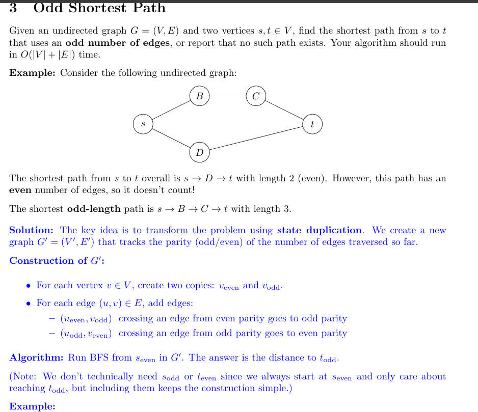
state duplication:将路径的奇偶性编码进入图里面
BFS才适合找最短路径

MBST:最大边值最小的生成树,MBST不一定是MST,但是MST一定是MBST

proof:假设不成立,MST删去最大边,cut一定可以用MBST中一个权重更小的边来替换,导致MST可以得到更小的总权重,矛盾

anscestor:可以考虑DFS的pre和postvisit关系

trees

找树的重心(centroid,一个点满足删除后剩下的所有子树节点小于二分之n)

algorithm:DFS,记录所有子树的大小,该点满足每个子树的size小于二分之n,除去该点为根的子树的剩余部分size也小于二分之n
proof:从根节点开始,每次往子树size大于二分之n的那边走(一定满足父方向小于二分之n),一定会停在一个点,但是这个点可能不唯一
应用:求彼此路径长度为k的点对,重心分治.

seperator

u-v seperator S:每条从u到v的路径都经过S中的元素

algorithm:BFS分层,记录距离,Si就是所有距离为i的点

2sat

In the 2SAT problem, you are given a set of clauses, where each clause is the disjunction
(OR)oftwoliterals (a literal is a Boolean variable or the negation of a Boolean variable).
You are looking for a way to assign a value true or false to each of the variables so that
all clauses are satisfied– that is, there is at least one true literal in each clause.
实际上可以转化为有向图强连通分量问题:
构造图:所有点代表一个变量和它的否,对一个clause a OR b,链接a否和b,b否和a,这样边(u,v)表示谓词u推v
思路:构建蕴含图,找强连通,拓扑排序强连通,重复将sink SCC所有字面量赋值true并删除该SCC

dynamic programming

shortest path in dag(revisited)

dag的一个突出特征就是其节点可以被线性化
在寻找最短路径的时候

$dist(v)=min_{(u,v)\in E}(dist(u)+l_{(u,v)})$

这代表我们将原本的问题分解为了几个子问题
dynamic programming:a problem is solved by identifying a collection of subproblems and tackling them one by one, smallest first,using the answers to small problems to help figure out larger ones, until the whole lot of themis solved.
动态规划中的dag是隐形的

longest increasing subsequence

problem:一个数字序列,要求找到最长的序列,满足序号越大,数字的值越大

建立dag:每个数字给一个node,任意两个node之间如果满足序号和数字的关系就添加一条边
L(j)=max(1+L(i))
如果想要能够重构出这条序列,在找L(j)的时候维护prev(j)=i即可
简单递归会大量地重复解子问题,通常分治的子问题规模减小很快

edit distance

两个单词的distance:各单词中间添加任意空格后相应位置不相同的位置个数最小和
solution:

subproblem:E(i,j)表示x字符串到i的子串和y字符串到j的子串
E(i,j)=min(E(i-1,j)+1,E(i,j-1)+1,diff(i,j)+E(i-1,j-1))
- 最右边只有三种情况:x为空,y为空,都不为空
basecase: E(0,j)=E(j,0)=j;

common subproblems:(前面的括号表示子问题的数目)

(linear) input:x1,x2…xn subproblem:x1,x2…xi
(O(mn)) input:x1,x2…xm & y1,y2…ym subproblem:x1,x2…xi&y1,y2…yj
(O(N2)) input:x1,x2…xn, subproblem:xi…xj

Knapsack(背包)

背包承重有限的情况下选出价值最大的搭配
实质上是资源受限条件下的选择问题
当我们看到正比于某个限制条件的时间复杂度的时候,这实际上是一个伪多项式,由于数字的表示,实际上对于输入长度是指数级的复杂度

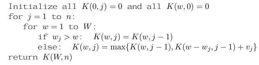
knapsack with repetition

$K(w)=max_{i:w_i\le w}(K(w-w_i)+v_i)$

其中w表示容量,k表示该容量下最大的价值

knapsack without repetition
we need to indicate whether it’s used,j means item 1 to j
memorization
DP是自底向上,记录式递归是自顶向下,两者理论复杂度相同,但是后者cache,function call有额外开销

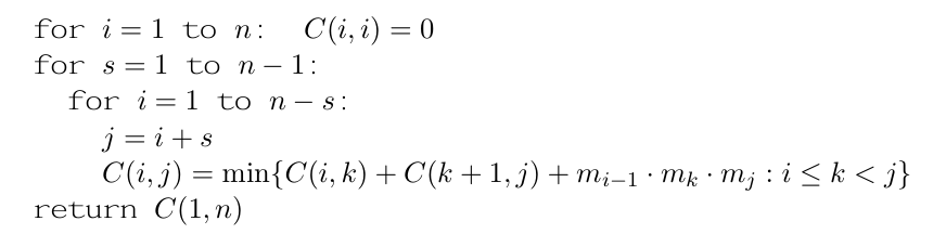
chain matrix multiplication

对m×n矩阵和n×p矩阵的乘积,一共mnp次乘积
区分:这里应该是区间dp,因为最后一次矩阵乘法可能发生在矩阵链的任意部分
用图画出来是个二叉树(构建最优树的子树一定最优,如果不最优就可以有别的更小)
alt text

shortest path

shortest reliable path:不仅总权重最小,还要求尽可能少的边(e.g:计算机网络,每次换边有可能导致丢失信息)
dist(v,i) represent the length from s to v using i edges

$dist(v,i)=min_{(u,v)\in G}(dist(u,i-1)+l(u,v))$

all pairs shortest path

for i =1 to n:
    for j =1 to n:
        dist(i,j,0) = ∞
for all (i, j) ∈ E:
    dist(i, j, 0) = `(i, j)
for k = 1 to n:
    for i = 1 to n:
        for j = 1 to n:
            dist(i, j, k) = min{dist(i, k, k − 1) + dist(k, j, k − 1), dist(i, j, k − 1)}

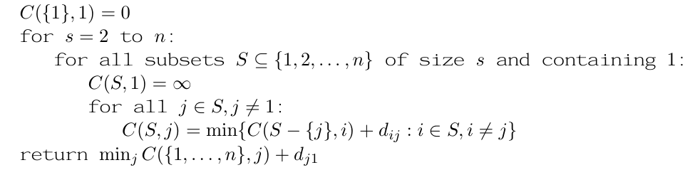
the traveling salesman problem
最小遍历所有点一次的总路径
C(S,j):the length of the shortest path from start to j and visit all the node in S

independent set in trees

idenpendent set of a graph:图中的节点,彼此之间没有边
图的解法很难,但是树的递归结构很良好的为其提供了dp解法
I(u)=以u为根节点的树的最大

$I(u)=max(1+\sum_{v\in grandchildren(u)}I(v),\sum_{v\in children(u)}I(v))$

disc&hw04

一个环中权重最大的边不可能属于最小生成树,如果属于可以移除而不影响连通性

三叉哈夫曼编码
lemma:任意最优三叉编码最多只有一个二叉节点,其他非叶子节点都是三叉
n为奇数:直接合并即可
n为偶数:第一步合并两个,后面都合并三个(若两个在更高的位置,更低位置的某个节点就可以接到第三个位置以减小总权重)
graph game(很多时候贪心策略比我想得简单)

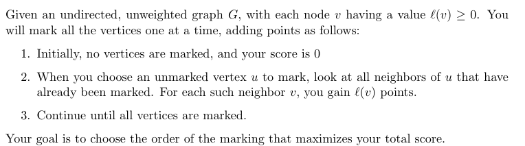
直接降序贪心,逐个标记就可以

#在python中只要有赋值语句就会被视为函数的局部变量
#所以要用nonlocal,才能在嵌套函数用外部的变量
def dfs_path(adj_list, s, t):
    """
    args:
        adj_list:List[List] = an adjacency list 
        s:int = an int representing the starting node
        t:int = an int representing the destination node

    return: 
        a list of nodes starting with s and ending with t representing an s to t path if it exists. 
        Returns an empty list otherwise
    """
    visited=set()
    tpath=[]
    target=t

    def explore(adj_list, curr):
        """
        implements the explore subroutine from DPV, which is used in DFS. feel free to delete this 
        function and use an alternative implementation if you prefer.

        args:
            adj_list:List[List] = an adjacency list 
            curr:int = the node currently being traversed
        
        return:
            None
        """
        nonlocal tpath
        visited.add(curr)
        tpath.append(curr)
        if curr==target:
            return True
        s=adj_list[curr]
        for node in s:
            if node not in visited:
                if explore(adj_list,node):
                    return True
        tpath.pop()
        return False
    # implement the dfs and path reconstruction here
    target=t
    if explore(adj_list,s):
        return tpath
    return []
#python set 为引用类型,每次要新建一个
def find_SCCs(adj_list):
    """
    args:
        adj_list:List[List[int]] = the adjacency list that represents our input graph
    return:
        List(Set(int, ...), ...) a list of sets where each set contains all the nodes 
            that belong to the corresponding SCC
    """
    visited=set()
    scc_list = []
    reversed=reverse_graph(adj_list)
    _,post=get_pre_post(reversed)
    post.reverse()
    def findSCC(node,SCC_com):
        SCC_com.add(node)
        visited.add(node)
        for nei in adj_list[node]:
            if nei not in visited:
                findSCC(nei,SCC_com)
    def traverseSCC(range_list):
        for node,_ in range_list:
            if node not in visited:
                SCC_com=set()
                findSCC(node,SCC_com)
                scc_list.append(SCC_com)
    
    traverseSCC(post)
    return scc_list
def bellman_ford(G, s, t):
    """
    使用 Bellman-Ford 算法查找最短路径。
    如果不存在路径或图中包含负权环，返回 []。
    """
    n = len(G)
    dist = [float('inf')] * n
    prev = [None] * n
    dist[s] = 0

    # 1. 进行 n-1 轮松弛
    # 每一轮尝试更新所有边。最短简单路径最多包含 n-1 条边。
    for i in range(n - 1):
        any_update = False
        for u in range(n):
            if dist[u] == float('inf'):
                continue
            # 假设 G[u] 格式为 (neighbor, weight)
            for v, weight in G[u]:
                if dist[u] + weight < dist[v]:
                    dist[v] = dist[u] + weight
                    prev[v] = u
                    any_update = True
        # 如果某一轮没有任何更新，说明已经收敛，提前退出以优化性能
        if not any_update:
            break

    # 2. 第 n 轮松弛：检测负权环
    # 如果在 n-1 轮之后还能更新，说明存在负权环
    for u in range(n):
        if dist[u] == float('inf'):
            continue
        for v, weight in G[u]:
            if dist[u] + weight < dist[v]:
                # 按照题目要求：如果存在负权环，返回空列表 []
                return []

    # 3. 检查终点是否可达
    if dist[t] == float('inf'):
        return []

    # 4. 构造路径并预防 MemoryError
    path = []
    curr = t
    visited = set() # 最后的防线：确保不会因为逻辑错误陷入死循环
    
    while curr is not None:
        if curr in visited:
            # 理论上前面的负权环检测应该已经拦截了这种情况
            return []
        path.append(curr)
        visited.add(curr)
        if curr == s:
            break
        curr = prev[curr]

    # 确保路径确实是从 s 开始的
    if not path or path[-1] != s:
        return []

    # 返回反转后的路径 [s, ..., t]
    return path[::-1]

backpropagation

普通的梯度计算方法太慢,反向传播实际上是一个动态规划

computational graph

source nodes:the input variables and constant
internal nodes:represent element-wise operation(log,exp,*.etc)
sink node:the output
前向传播就是仅仅以拓扑排序遍历整个有向无环图(O(V+E))

algorithm

alt text
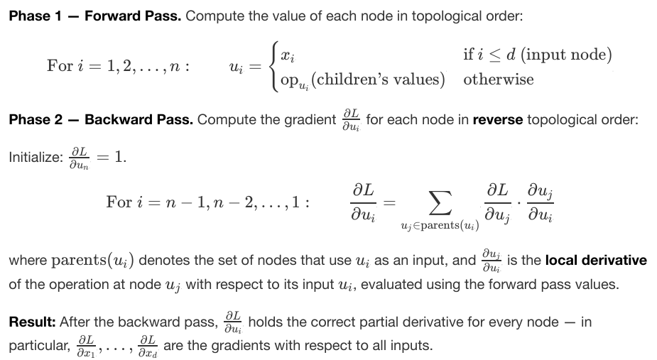
实际上就是加权路径求和

hw&disc5

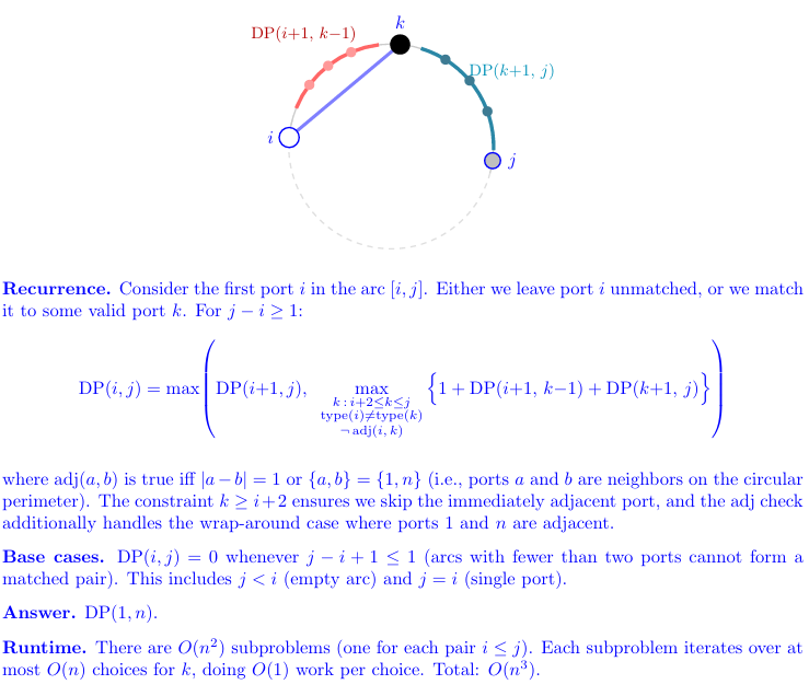
是否需要从中间断开来求:是才是区间dp

circuit design:电线不能相交,这就将区间分成了两个不能相交的部分
longest common sequence
对xi和yj:要么匹配,要么x++,要么y++
motel
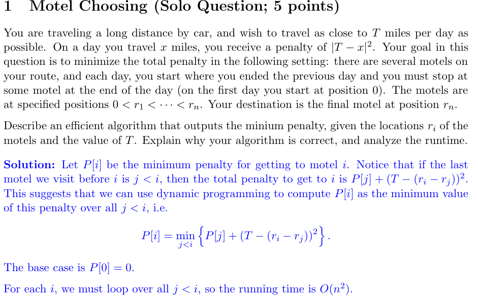
计算runtime:状态维度(子问题数)乘以转移耗时(求解子问题的)
证贪心:交换参数法,始终领先法(局部最优必然导致全局最优,min max)
扔鸡蛋问题:k个鸡蛋,扔最少次数找到n层楼中刚刚好不会打碎的层数
区间dp:很多时候是中间寻找一个状态

$f(i,j)=1+min(max(f(x-1,j-1),f(i-x,j-1)))$

def edit_distance(x, y):
    n = len(x)
    m = len(y)
    # 初始化 (n+1) x (m+1) 矩阵,区分索引和长度
    matrix = [[None] * (m + 1) for _ in range(n + 1)]

    def dp(i, j):
        # 基础情况：如果其中一个字符串长度为 0
        if i == 0:
            matrix[i][j] = j
            return j
        if j == 0:
            matrix[i][j] = i
            return i
        
        if matrix[i][j] is not None:
            return matrix[i][j]
        
        # 递归计算
        # 1. 删除 (x[i-1])
        res1 = dp(i - 1, j) + 1
        # 2. 插入 (y[j-1])
        res2 = dp(i, j - 1) + 1
        # 3. 替换或匹配
        # 注意：i, j 表示长度，对应的字符索引是 i-1, j-1
        cost = 0 if x[i-1] == y[j-1] else 1
        res3 = dp(i - 1, j - 1) + cost
        
        res = min(res1, res2, res3)
        matrix[i][j] = res
        return res

    # 填充矩阵
    dp(n, m)

    # 回溯构造字符串 (使用循环比递归更稳健)
    x_padded, y_padded = "", ""
    i, j = n, m
    while i > 0 or j > 0:
        current = matrix[i][j]
        
        # 尝试从 “替换/匹配” 方向回来
        if i > 0 and j > 0:
            cost = 0 if x[i-1] == y[j-1] else 1
            if current == matrix[i-1][j-1] + cost:
                x_padded = x[i-1] + x_padded
                y_padded = y[j-1] + y_padded
                i -= 1
                j -= 1
                continue
        
        # 尝试从 “删除” 方向回来
        if i > 0 and current == matrix[i-1][j] + 1:
            x_padded = x[i-1] + x_padded
            y_padded = '-' + y_padded
            i -= 1
        # 尝试从 “插入” 方向回来
        else:
            x_padded = '-' + x_padded
            y_padded = y[j-1] + y_padded
            j -= 1

    return (x_padded, y_padded)

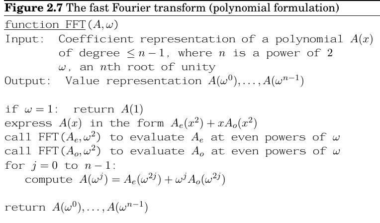
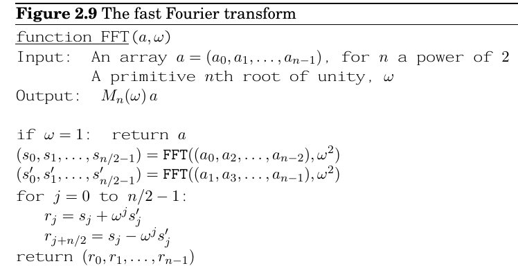
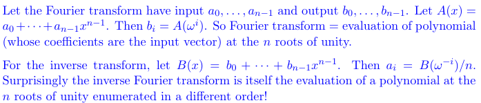
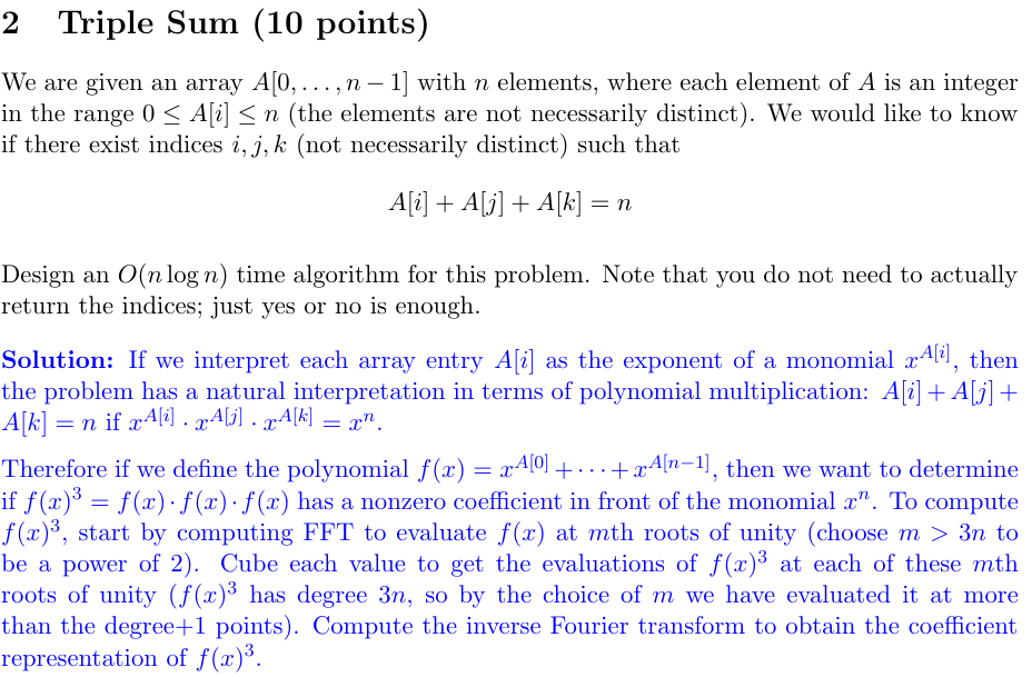
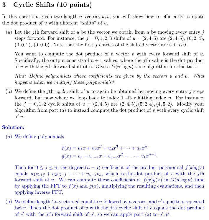
fast fourier transform

傅里叶变换也可以被解释为多项式在多个点求值
多项式乘法和快速大整数乘法结构类似:只要将x换为2
linear time invariant system(线性时不变系统):对信号和的响应为对各信号响应的和,不同时刻输入信号的输出一样
impulse response(单位脉冲):对t=0时脉冲的响应,只要知道这个就能知道系统的响应

$\begin{aligned} b (t)\gets \delta(t)\text{ system gives response b }\\ c(k)=\sum_{i=0}^k a(i)b(k-i)\text{ the output of system at time k response to a} \end{aligned}$

an alternative representation

fact:a polynomial of degree d is determined by its value at any d+1 points

说明:点值向量可以由自变量的幂构成的矩阵和系数向量相乘得到,只要自变量不取相同的值,矩阵可逆
so it has two representation
coefficient:
the values A(x0),…A(xd)

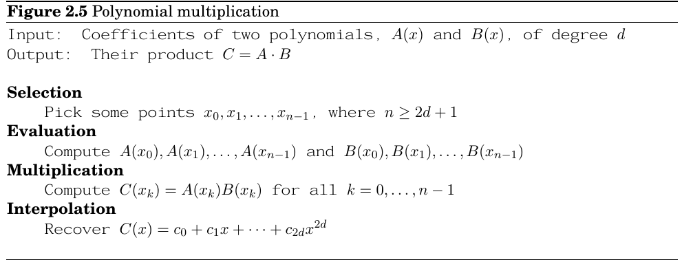
evaluation by divide and conquer

核心思想:利用复数域对称性复用计算结果
alt text

interpolation(插值)

value Representation=FFT(coefficient,omega)
coefficient Representation=1/n FFT(value,1/omega)
因为FFT矩阵是列正交的,其逆非常好求,并且乘矩阵实际上是基变换(rigid rotation)
alt text

parallel algorithm

the work-span model

推理并行计算的一种方法:视为一种scheduling,也可以视为一个有向无环图

work and span

work:T1,单处理器所需时间,也即dag中的所有点
span:T无穷,无穷多处理器也至少需要的时间,dag中的最长有向路径(also called critical path)
speedup:sp为T1除TP
efficiency:T1/pTP
parallelism:T1/T无穷

brent’s rule

$T_p\le \frac{T_1}{p}+T_{\infty}$

case study

integer multiplication

整数乘法通常是计算各部分的积最后求和
实际上加是很慢的,因为每一位在二进制下是否要进位都依赖前一位,有向无环图看起来像一条线
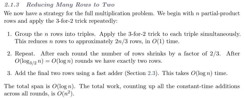
central idea:将三个数相加变为两个数的和,在多处理器常数时间下
X+Y+Z=S+C
X,Y,Z的第k位求和,其sum bit 可直接赋给sk,carry bit(进位)直接赋给c(k+1)
alt text

parallel prefix(scan)

$y_k=x_1\odot x_2\odot ...x_n$

其中仅仅只要求这种抽象运算有结合律即可
算法:相邻两个结合来算(没有依赖性,可并行)
递归执行,最后结果分奇偶再来就行

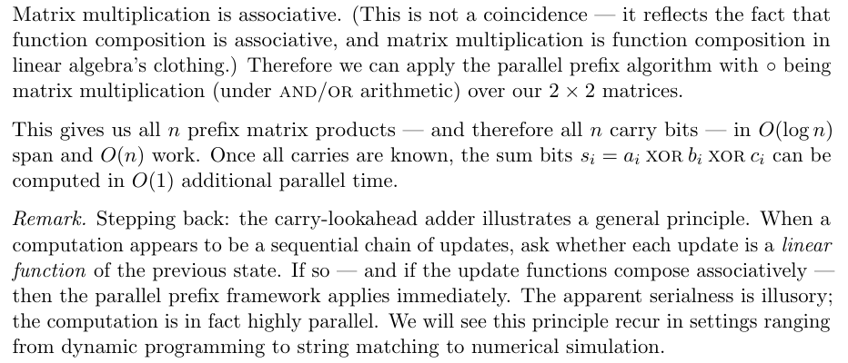
Carry-Lookahead Addition

$\begin{aligned} g_i(generate)&=a_i AND b_i\\ p_i(propagate)&=a_i XOR b_i\\ c_{i+1}&=g_i OR (p_i AND c_i) \end{aligned}$

我们可以使用矩阵形式更明显地消除递归依赖
(使用AND代替乘法和使用OR代替加法)

$\begin{bmatrix} c_{i+1}\\ 1 \end{bmatrix}= \begin{bmatrix} p_i & g_i\\ 0 & 1 \end{bmatrix} \begin{bmatrix} c_{i}\\ 1 \end{bmatrix}$

alt text

disc&hw6

证贪心:设最优的和贪心结果有最大overlap,推出还有更大
relax:更新d基于其邻居的d
max contiguous array sum:

$\begin{aligned} solve(A)=max(solve(A_L),solve(A_R),inter)\\ inter=\text{Maximum sum of suffix of }A_L+\text{Maximum sum of prefix of } A_R \end{aligned}$

gradient descent

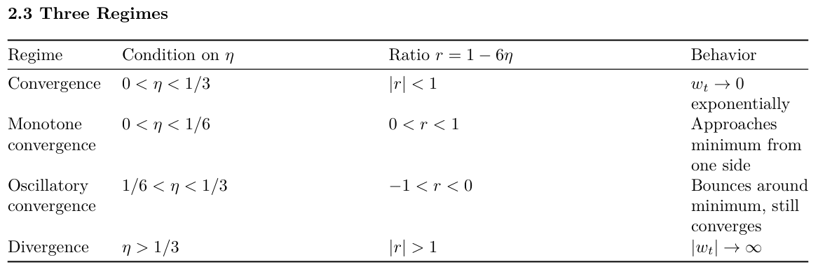
学习率设置对收敛的影响(原函数越steep学习率越应该较小)
alt text

Smoothness and the Descent Lemma

L-smoothness

$\forall x,y\in \mathbb{R}^d,||\nabla f(x)-\nabla f(y)||\le L\times ||x-y||$

对多元二阶可导的函数,L可以直接取函数黑塞矩阵的最大特征值

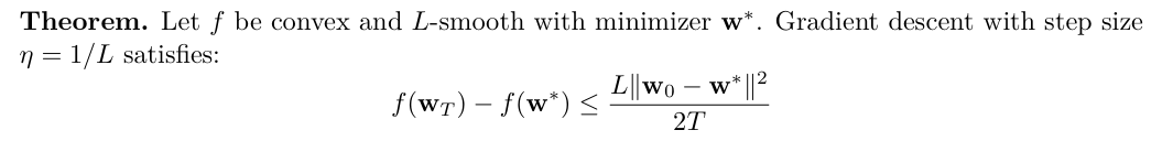
descent lemma
下式设置学习率为L的倒数可以取得相当好的效果

$f(w_{t+1})\le f(w_t)-\eta(1-\frac{L\eta}{2})||\nabla f(w_t)||^2$

alt text

disc&hw7

gradient checkpoint

以时间换空间,不保存计算图中所有中间计算结果,而是仅保留部分
alt text

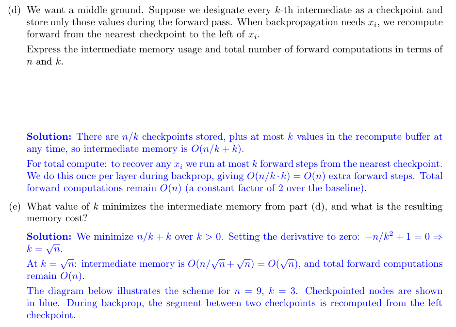
数值之和=>指数之和

alt text

解法:识别目标(滑动求和),加法乘法变指数,循环变链(两倍链条)

fft实现

np中的虚数单位是1j

import numpy as np

def fft(coeffs, roots):
    n = len(coeffs)
    
    # 1. 基准情况：如果多项式只有一个系数，直接返回该系数
    if n == 1:
        return [coeffs[0]]
    
    # 2. 拆分：奇数项和偶数项
    # 注意：这里长度会减半，从 n 变成 n/2
    coeffs_even = coeffs[0::2]
    coeffs_odd = coeffs[1::2]
    
    # 3. 准备子问题的单位根：(w^k)^2 = w^{2k}，即 n/2 次单位根
    # 我们只需要前 n/2 个
    half_n = n // 2
    new_roots = roots[0::2] # 步长为2，取出的刚好是 w^0, w^2, ...
    
    # 4. 递归求解子问题
    ae = fft(coeffs_even, new_roots)
    ao = fft(coeffs_odd, new_roots)
    
    # 5. 合并结果 (Butterfly Operation)
    # 利用对称性：P(w^k) = E(w^{2k}) + w^k * O(w^{2k})
    #           P(w^{k+n/2}) = E(w^{2k}) - w^k * O(w^{2k})
    ret = [0] * n
    for j in range(half_n):
        # 旋转因子
        w_j = roots[j]
        # 合并前半部分
        ret[j] = ae[j] + w_j * ao[j]
        # 合并后半部分 (利用 w^{j+n/2} = -w^j)
        ret[j + half_n] = ae[j] - w_j * ao[j]
        
    return ret

Linear programming

Linear programming describes a broad class of optimization tasks in which both the constraints and the optimization criterion are linear functions.

introduction

核心定义 (The Core Concept)
线性规划是一种优化技术，其目标是在满足一组线性约束（等式或不等式）的前提下，最大化或最小化一个线性目标函数。

变量 ( $x_i$ )：通常为实数。
目标函数：例如 $\max c_1x_1 + c_2x_2 + \dots + c_nx_n$ 。
约束条件：变量必须满足的限制，如 $a_1x_1 + a_2x_2 \leq b$ 。

几何视角 (The Geometry of LP)
理解 LP 的几何意义是掌握其算法的基础：

可行域 (Feasible Region)：所有满足约束条件的点 $(x_1, x_2, \dots, x_n)$ $(x_{1}, x_{2}, \dots, x_{n})$ 的集合。
- 在 2D 中是一个凸多边形。
- 在 3D 中是一个凸多面体 (Polyhedron)。
- 在 $n$ 维中是一个多胞形 (Polytope)。
等值线/面 (Contour Lines/Planes)：目标函数值等于常数 $c$ 的线或面。随着 $c$ 的增大，这条线/面会在空间中平行移动。
顶点属性 (Vertex Property)：
- 核心结论：最优解必然在可行域的顶点处取得。
- 如果最优解不唯一（例如目标函数与某条边平行），则整条边上的点都是最优的，但其中必然包含顶点。

特殊情况：

不可行 (Infeasible)：约束条件互相矛盾（例如 $x \leq 1$ 且 $x \geq 2$ ），可行域为空。
无界 (Unbounded)：约束太松，目标函数可以达到无穷大（例如 $\max x+y$ 且 $x,y \geq 0$ ）。
单纯形法逻辑 (Simplex Method Logic)
单纯形法是求解 LP 最常用的算法（由 George Dantzig 提出）：
起点：从可行域的一个顶点开始（通常是原点）。
迭代（爬山）：观察相邻的顶点。如果某个相邻顶点的目标函数值更高，就移动到该顶点。
停止条件：当所有邻居的值都不如当前顶点时，宣布达到最优。
局部 vs 全局：由于可行域是凸的，局部最优即为全局最优。
建模实战与技巧 (Modeling Examples)
通过文中例子，复习如何将实际问题转化为数学语言：

A. 生产调度问题（如地毯厂）

时间维度变量：对于 12 个月的问题，需要为每个月定义变量（如 $w_i$ 工人数、 $s_i$ 库存数）。
状态转移约束：
- 工人平衡： $w_i = w_{i-1} + h_i - f_i$ （本月工人 = 上月 + 雇佣 - 解雇）。
- 库存平衡： $s_i = s_{i-1} + x_i - d_i$ （本月库存 = 上月 + 产量 - 需求）。
整数性问题：LP 解可能是小数（如雇佣 10.6 人）。虽然可以四舍五入，但对于小数值变量，四舍五入可能偏离最优解。寻找最优整数解的问题称为整数线性规划 (ILP)，这是 NP-hard 问题。

B. 网络带宽分配

流量建模：为每条可能的路径定义一个变量。
容量约束：所有经过某条物理边 (Edge) 的路径流量之和 $\leq$ 该边的总带宽。
需求约束：每对用户间的总流量 $\geq$ 最低需求。

对偶性 (Duality) - 验证最优解

直观理解：如果你想证明你的利润 $3100$ 是最高的，你可以通过将原始约束条件进行线性组合（乘以适当的系数并相加），推导出一个形如 $Profit \leq 3100$ 的不等式。
乘法器 (Multipliers)：这些用于组合约束条件的系数本身构成了另一个 LP 问题，称为对偶问题。

线性规划的变体与归约 (Variants & Reductions)
在考试或编程中，常需要将各种形式的 LP 转化为标准型 (Standard Form)：

原始形式	转化方法
最大化问题 (Max)	目标函数乘以 $-1 \Rightarrow$ 转为最小化问题 (Min)
不等式约束 ( $\leq b$ )	引入松弛变量 (Slack Variable) $s \geq 0$ ，变为 $Ax + s = b$
等式约束 ( $= b$ )	拆分为两个不等式： $Ax \leq b$ 和 $Ax \geq b$
无符号限制变量 ( $x$ )	替换为 $x = x^+ - x^-$ ，其中 $x^+, x^- \geq 0$

矩阵表示法 (Matrix Notation)
为了简洁和计算，LP 通常写为：

目标函数： $\max \mathbf{c}^T \mathbf{x}$
约束条件： $A\mathbf{x} \leq \mathbf{b}$ $A x \leq b$ 和 $\mathbf{x} \geq 0$ $x \geq 0$
- $A$ 是约束系数矩阵。
- $\mathbf{b}$ 是资源限制向量。
- $\mathbf{c}$ 是利润/成本系数向量。

复习思考题：

为什么线性规划的最优解一定在顶点上（凸多面体,往点移动至少能做到不变）。
如果在爬山过程中，所有邻居的利润都和当前顶点一样，单纯形法会停止吗？这说明了什么(会,最优解无穷多个)
松弛变量的物理意义是什么（它通常代表未使用的资源,某松弛变量大于零对应的原变量增加也不会增加利润）。
为什么整数线性规划比普通线性规划难得多(舍入失效,同时可能不凸了)

duality

alt text
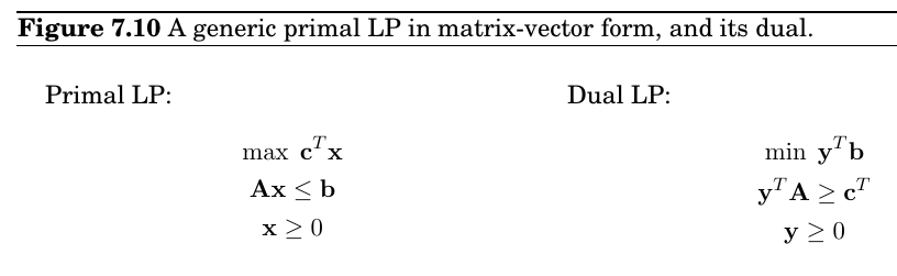
等式约束对应的对偶变量不一定要求非负

理解:乘子法
我们通过对原问题的不等式约束的线性组合凑出目标函数的一个上界
对线性组合求最小值的结果即可精确确定原目标函数的上界
e.g:
最大流等价于最小割
找最小路径:物理上构建出这个图,从s到t的最短路径实际上可以通过让s尽可能离t远得到

Klee-Minty Example

对于有n个变量和m个不等式约束的线性规划问题,每个点都是由n个tight不等式(a.k.a. 刚好满足)
每两个相邻的点实际上共享n-1个约束,从一个点移动到另一个实际上就是loosen一个约束,变紧另一个约束
坐标变换:在某个顶点u的时候,将其移动到坐标原点,这样当变换后目标系数均为负,就是最大的
实际算法

Procedure Simplex(max c⊤x s.t. Ax ≤ b, x ≥ 0):

1.  Let u be any feasible vertex.
2.  while true: 
    • Rewrite the LP in local coordinates y centered at u; theobjective becomes cu +¯ c⊤y. 
    • if ¯ci ≤ 0 for all i: return u (optimal!) 
    • Pick i with ¯ci > 0
    • Increase yi until a new constraint aj · x = bj becomes tight. 
    • u←the new vertex.

找初始点
alt text

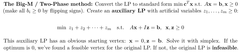
如果超过n个不等式约束到了一点可能导致变成环,一点轻微扰动就能够解决

cs170&DPV

Arithmetic Algorithms

multiplication

recurrence relation

mergesort & median

dis&hw1

fast matrix multiplication

graph

depth first search

strongly connected component

disc&hw2

path in graphs

shortest path with negative edge

shortest in dags

Greedy

minimum spanning tree

huffman encoding

horn formulas

set cover

disc&hw3

trees

seperator

2sat

dynamic programming

shortest path in dag(revisited)

longest increasing subsequence

edit distance

Knapsack(背包)

chain matrix multiplication

shortest path

independent set in trees

disc&hw04

backpropagation

computational graph

algorithm

hw&disc5

fast fourier transform

an alternative representation

evaluation by divide and conquer

interpolation(插值)

parallel algorithm

the work-span model

work and span

brent’s rule

case study

integer multiplication

parallel prefix(scan)

Carry-Lookahead Addition

disc&hw6

gradient descent

Smoothness and the Descent Lemma

disc&hw7

gradient checkpoint

数值之和=>指数之和

fft实现

Linear programming

introduction

duality

Klee-Minty Example